Wombling is an approach for detecting discontinuities or boundaries within spatial data. The general procedure is that individual boundary elements (potential boundaries) are identified by the spatial configuration of the data points (see below). Each boundary element is assigned a magnitude of change across the element (and for certain types of wombling, a vector/direction of change as well). Adjacent boundary elements which meet specified criteria (e.g., high magnitude of change, similar direction, etc.) are combined into subboundaries which represent the areas of greatest change/discontinuity within the data set. The exact nature of the wombling analysis depends on two independent sets of contrasts: first, are the magnitudes of change based on pairs of data points (often called categorical wombling) or based on more than two data points (often called continuous wombling); second, are the spatial locations scattered or spread evenly across a surface. PASSaGE uses separate interfaces for performing Wombling analysis on scattered and surface data, although most of the options are identical. The differences between continuous and categorical wombling are described below.
In continuous wombling, boundary elements are point positions identified through sets of more than two data points. For surface data, boundary elements are located at the centroid of the four data points making up a square (or put another way, the common corner of each set of four cells in the surface). This is often referred to as lattice wombling. Boundary elements are considered adjacent if they follow one of three chess rules: rook movements (adjacent elements are vertically or horizontally contiguous), bishop movements (adjacent elements are diagonally contiguous), or queen movements (adjacent elements are horizontally, vertically, or diagonally adjacent). For scattered data, boundary elements are located at the centroid of each triangle identified through a Delaunay triangulation. This is often referred to as triangulation wombling. Boundary elements are considered adjacent if their triangles share a common edge, i.e., two of the three surrounding data points are common to both elements. In both cases, the values associated with the data points surrounding the element are used to estimate the direction and magnitude of change associated with the element as the first partial derivative of the variable in both x and y directions.
The magnitude is measured as
where
![]()
for lattice wombling, with ZA, ZB, ZC and ZD being the value associated with the four data points (cells) surrounding the element and the x/y coordinates rescaled to range from 0 to 1. For triangulation wombling,
![]()
where
 .
.
For both cases the direction of the vector describing the change is calculated as
 .
.
Adjacent boundary elements are connected into subboundaries if the pass three criteria. (1) both elements must be in the top X% (as set by the user) of all elements with respect to the magnitude of the change. (2) The difference in direction of the gradients of the two elements must be less than a specified angle. This prevents the connection of boundary elements which indicate opposing gradients. (3) the angular difference between the bearing which connects the boundary elements and the bearing of the gradient of the elements should be above a specified threshold. As a rule, boundary elements should not be connected along the gradient itself, but (optimally) perpendicularly across the gradient.
(a)  (b)
(b) 
Illustration of similar bearing issues. (a) the vectors associated with the two boundary elements point in a similar direction and therefore might be combined into a subboundary. (b) the vectors associated with the two boundary elements point in opposite directions and likely should not be combined in a subboundary.
(a)  (b)
(b) ![]()
Illustration of difference in vector issues. (a) the bearing of the subboundary is vertical while the gradient of change is horizontal; the connected subboundary is perpendicular to the direction of change. (b) the bearing of the subboundary is in roughly the same direction as the gradient of change; a subboundary consisting of these elements would not accurately reflect a boundary between areas of different value.
In categorical wombling, boundary elements are line segments identified through contrasts between pairs of adjacent data points. For surface data these elements are simply the edges of each cell. For scattered data, a tessellation is constructed to represent the boundaries between each point. Boundary elements are considered adjacent if they have overlapping endpoints.
(a)  (b)
(b) 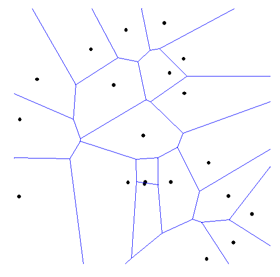
Examples of boundary elements for categorical wombling. (a) For surface data, each edge between adjacent cells is a boundary element. (b) For scattered data, a tessellation is used to identify boundary elements.
The magnitude of change for each element is calculated simply as the distance (using any standard distance measure for multivariate data) between the data points on either side of the element. Unlike continuous wombling, there is no vector or direction of change associated with an element. Adjacent elements are connected into subboundaries if both elements are in the top X% (as set by the user) of change based on this distance. Note that "categorical" wombling can be performed on continuous data since the magnitude of change can be based on any multivariate distance measure, and is thus, strictly speaking, not restricted to categorical data.